
王帅 , 徐涵秋, 施婷婷
1.福州大学环境与资源学院,福建 福州 350116
Wang Shuai, Xu Hanqiu, Shi Tingting
中图分类号: P237;TP7
文献标识码: A
文章编号: 1001-8166(2018)06-0641-12
通讯作者:
收稿日期: 2017-10-27
修回日期: 2018-05-16
网络出版日期: 2018-06-20
版权声明: 2018 地球科学进展 编辑部
基金资助:
作者简介:
First author:Wang Shuai (1992-), male, Fuyang City, Anhui Province, Master student. Research areas include remote sensing of resources and environment. E-mail:wswin8@hotmail.com
作者简介:王帅(1992-),男,安徽阜阳人,硕士研究生,主要从事资源环境遥感研究.E-mail:wswin8@hotmail.com
展开
摘要
针对国产GF-1 WFV2传感器,提出一种缨帽变换系数的推导方法。利用全国范围内不同地区的18幅GF-1影像和5幅同步的Landsat 8影像,选择了大量覆盖不同地物类型的典型样本并分析光谱变化特征。在此基础上,用3幅Landsat 8同步影像对湿度分量回归,然后再用施密特正交化方法依次推导出两两正交的亮度分量和绿度分量。结果显示,推导的前2个分量能解释缨帽变换总变化量的97%以上,前3个分量能解释总变化量的99%以上。针对不同区域影像的实验结果表明,各分量都具有很好的稳定性,而不同分量之间的散点图也都有相似的分布特征,说明该系数有很好的适用性。与验证用的Landsat 8同步影像对比后发现,推导的缨帽变换结果与Landsat 8相应的分量之间都有很好的相关性和一致性,尽管2种传感器波段设置及光谱响应能力不同,但相关性仍高达0.9。对GF-1 WFV1,WFV3和WFV4传感器影像的实验结果表明,针对GF-1 WFV2传感器提出的缨帽变换系数,也可以很好地应用在WFV3和WFV1传感器上,但不建议在WFV4传感器上使用。
关键词:
Abstract
Aiming at GF-1 WFV2 sensor, a method for deriving Tasseled Cap Transformation (TCT) coefficients was proposed in this paper. Based on 18 GF-1 images and 5 synchronous Landsat 8 images of different regions throughout the country, a large number of typical samples covering different ground types were selected, and the spectral characteristics of these samples were then analyzed. On this basis, the wetness component of the TCT was retrieved by the regression using three Landsat 8 and WFV2 synchronous images. The orthogonal brightness and greenness components were then derived with the Gram-Schmidt orthogonalization method. The results showed that the derived first two components can explain more than 97% of total variation, and the first three components can explain more than 99% of the total variation. The experimental results from different regions showed that each component had good stability, and the scatter-plots of different components also exhibited similar distribution patterns. This indicates that the derived coefficients have good applicability. Compared with the validation images, the results of TCT are well correlated with corresponding Landsat 8 components. Although these two sensors have different band settings and different spectral responses, their correlation coefficient is still as high as 0.9. The application results for GF-1 WFV1, WFV3 and WFV4 showed that the coefficients derived from WFV2 sensor can also be used for WFV3 and WFV1 sensors, but they are not recommended for WFV4 sensor.
Keywords:
缨帽变换(Tasseled Cap Transformation,TCT)是一种经验性的线性正交变换,最早由Kauth等[1]在研究农作物的生长期变化时提出,现在已被广泛应用在农业信息提取、农作物变化监测、遥感生态评估、植被制图、森林分类和生物量反演等众多领域[2,3,4,5,6,7,8,9],在遥感影像融合、图像解译等方面也具有重要的应用价值[10,11]。但是,由于不同传感器的波段设置及光谱响应特征的差异,尽管不同地物类型有着相对稳定的光谱特征,但它们在不同传感器光谱空间中的分布特征并不完全相同,因此从光谱空间到缨帽变换空间的变换矩阵仍取决于特定的传感器,从而导致根据某种传感器开发的缨帽变换系数无法直接代入其他的传感器数据。正因为如此,国内外学者针对不同卫星传感器的缨帽变换系数推导展开了大量的研究。
Kauth等[1]最早提出了针对Landsat MSS的缨帽变换系数,并指出农作物区域的影像在Landsat MSS的光谱空间中主要呈三角形分布在亮度线和绿度线组成的平面上。Crist等[12,13]对Landsat TM数据分析后发现,地物在TM光谱空间中主要分布在垂直的2个平面及其之间的过渡带上,并用主成分变换和坐标轴旋转的方法提出了TM的缨帽变换系数。但与MSS不同的是,TM缨帽变换的第3分量对土壤湿度很敏感[13],因此被称为湿度分量。Huang等[14]用与Crist类似的方法,提出了针对Landsat ETM+卫星表观反射率的缨帽变换系数。在Landsat 8卫星发射以后,Baig等[15]以Landsat TM传感器缨帽变换后的特征空间为目标,利用普鲁克分析(Procrustes Analysis)算法将Landsat 8 OLI经过主成分变换的结果旋转到TM的缨帽变换空间,得到了Landsat 8 OLI的缨帽变换系数。此后,Liu等[16,17]和李博伦等[18]针对Landsat 8 OLI传感器各自提出了不同的变换系数。除了Landsat系列卫星,国外学者还分别提出了其他卫星系列的缨帽变换系数。Yarbrough等[19]分别求出了ASTER基于卫星表观辐射亮度和表观反射率的缨帽变换系数,并认为后者在变化检测中有更好的效果。Lobser等[8]把缨帽变换概念拓展到MODIS 经过双向反射分布函数校正的数据(Nadir BRDF-Adjusted Reflectance)上,同样用主成分变换结合普鲁克算法求出了MODIS的缨帽变换系数。Horne[20]提出了IKONOS的缨帽变换系数并指出该系数同样适用于IKONOS多光谱与全色波段的融合影像。Yarbrough等[21]针对QuickBird 2影像用3种不同的方法推导出了相似的变换结果,并推荐使用施密特正交化(Gram-Schmidt Orthogonalization Process)方法。Verdin等[22] 、Silva[23]和Ivits等[24]分别提出了针对SPOT1,SPOT2和SPOT5传感器的缨帽变换系数,后者还研究了SPOT5缨帽变换各分量对季节和地理位置的依赖性。
随着国产卫星相继升空,国产卫星数据的缨帽变换系数研究也逐渐展开,Sheng等[25]提出了CBERS-02B CCD传感器的缨帽变换系数,并将第3分量称为蓝度分量(Blueness)。Chen等[26]提出了HJ-1A/B CCD传感器的缨帽变换系数,并指出HJ-1A/B 4个CCD传感器的缨帽变换分量有着几乎相同的方向。当前,ZY-3,GF-1,GF-2,GF-4和GF-3等国产卫星已陆续升空并投入使用,然而,与高分系列卫星相对应的缨帽变换公式却迟迟未见提出,影响了卫星数据在农业信息提取和农业监测等方面更广泛的应用。因此,如何推导针对国产高分系列卫星传感器的缨帽变换系数成了迫切需要解决的问题。由于GF-1 WFV (Wide Field of View)传感器数据现已可以免费下载,因此具有广阔的应用前景。鉴于此,本文以GF-1 WFV2传感器为例,利用全国范围内的18景WFV2多光谱影像,并结合5景同步的Landsat 8 OLI影像,研究了基于GF-1 WFV2传感器表观反射率的缨帽变换推导方法并提出了相应的变换系数,以期能够促进GF-1卫星数据更广泛的应用,并为ZY-3,GF-2和GF-4等国产高分辨率卫星的缨帽变换研究提供参考。
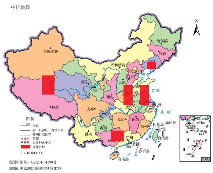
为了使推导的缨帽变换系数具有普适性,本文在全国范围内的不同区域选取了18幅覆盖不同生长季节的GF-1 WFV2影像,并根据GFV-1与Landsat 8的部分重叠轨道,挑选了5幅无云的Landsat 8同步影像(表1),分别用来做湿度分量的回归和缨帽变换结果的检验。影像的时间跨度为2015/05/20-2017/04/01,区域范围包括我国中部、东部沿海、西部、南方及东北地区(图1)。
表1 数据源列表
Table 1 Source lists of data
| 所属 区域 | 地点 | 成像 日期 | GF-1 产品号 | Landsat 8 列/行 | |
|---|---|---|---|---|---|
| 实验 影像 地区 | 中部 地区 | 驻马店、信阳 | 20151020 | 1116843 | |
| 开封、商丘、亳州 | 20160504 | 1562284 | 123/36 | ||
| 驻马店、信阳、阜阳 | 20160908 | 1562295 | 123/37 | ||
| 驻马店、信阳、阜阳 | 20160908 | 1813878 | |||
| 东部 地区 | 日照市 | 20160429 | 1552922 | 120/36 | |
| 南京、滁州 | 20160429 | 1552923 | |||
| 南方 地区 | 柳州、来宾 | 20161216 | 2047782 | ||
| 玉林、贵港 | 20170401 | 2277357 | |||
| 柳州、贺州 | 20170401 | 2277356 | |||
| 西部 地区 | 乌兰乌拉湖,西北 | 20160721 | 1712329 | ||
| 乌兰乌拉湖,西北 | 20161117 | 1970495 | |||
| 东北地区 | 营口市 | 20160507 | 1569457 | ||
| 验证 影像 地区 | 中部 地区 | 聊城、濮阳 | 20160504 | 1562286 | 123/35 |
| 驻马店、信阳、阜阳 | 20160516 | 1586464 | |||
| 东部地区 | 连云港、淮安 | 20160429 | 1552914 | 120/37 | |
| 南方地区 | 贺州、梧州 | 20161228 | 2093687 | ||
| 西部地区 | 乌兰乌拉湖,西南 | 20161117 | 1970493 | ||
| 东北地区 | 营口市 | 20160919 | 1839479 |
从中国资源卫星应用中心(http:∥www.cresda.com/CN/)下载的GF-1影像是Level 1A级别,其空间参考系是地理坐标系,需要将其投影到常用的UTM投影坐标系中。采用卫星影像自带的RPC文件,利用ENVI 5.3中的 “RPC Orthorectification Workflow”和“Enhanced RPC Orthorectification Using Reference Image”进行基于RPC的正射校正,采样分辨率设置为16 m。缨帽变换系数的推导可以基于影像的灰度值,也可以基于卫星入瞳处的表观反射率。由于前者会受到太阳光照几何条件(如日地距离、太阳天顶角等)的影响,将其拓展应用到其他影像上时可能会出现不确定性[14],因此,本文的缨帽变换是基于卫星表观反射率来推导的,所以数据的预处理就是将影像的灰度值反演成卫星的表观反射率。利用公式(1)和公式(2)可以将GF-1影像的灰度值转换到传感器入瞳处的表观反射率。
式中:Lλ是传感器接收到的辐射亮度;Gain和Offset分别是传感器定标参数的增益值和偏置值;DN(Digital Number)值为遥感影像上像元的灰度值;Es是波段太阳辐照度,均从资源卫星应用中心的官方网站获取;d是日地天文距离,可从参考文献[27]中查找;θs为太阳天顶角,可从影像的头文件中获取,或者根据影像成像时间和成像地点的中心经纬度,从美国国家海洋和大气管理局(National Oceanic Atmospheric administration,NOAA)的Solar Calculator网站 (https:∥www.esrl.noaa.gov/gmd/grad/solcalc/index.html)计算得到。考虑到传感器的信号衰减及国产卫星地面场地定标实验频率的限制,经咨询中国资源卫星应用中心定标人员和负责人,定标参数的选择应遵循以下原则:6月前获取的影像采用前一年的定标系数,6月后获取的采用当年的定标系数。
由于从USGS下载的Landsat 8影像是L1T级别,已经做过地形数据参与的几何精校正,因此只需做辐射校正即可(公式(3))。
式中:Mρ为波段λ的反射率调整因子;Aρ为波段λ反射率调整参数,都可以在MTL头文件中找到;Qcal为影像的DN值;θs为成像时的太阳天顶角[28,29]。
缨帽变换是从地物的光谱空间到特征空间的一种正交变换,它根据多光谱遥感中土壤、植被等地物信息在光谱空间中的分布结构特征将其投影到缨帽变换空间中,并且能减少光谱维度,将信息集中在少数几个特征空间上。其定义为:
u=Ax+r,(4)
式中:u是缨帽变换后的向量;A是单位正交矩阵,亦即缨帽变换的系数矩阵;x是影像的灰度值或者传感器的表观反射率;r作为偏移向量是为了避免变换后的结果出现负值。
当前针对缨帽变换系数的推导主要有2种方法,一种是利用施密特正交化的方法,这也是Kauth和Thomas在研究MSS缨帽变换时首先使用的方法,后来常被用在4波段传感器的缨帽变换推导中,Jackson[30]对该方法进行了详尽的描述。另一种是基于统计思想的主成分变换法,该方法多用在有较多波段(波段数通常大于4)的传感器上,可以避免施密特正交化繁琐的计算过程。考虑到GF-1 WFV传感器只有4个波段,同时为了避免主成分变换方法中旋转角度的不确定性,本文选择用施密特正交化的方法来推导WFV2传感器的缨帽变换系数。
为了得到第1个缨帽变换系数(亮度分量),首先要确定土壤线在光谱空间的方向,并将其作为亮度分量的方向。在4维光谱空间中,至少需要2个典型的土壤样本才能确定土壤线的方向向量,每个土壤样本可以看作光谱空间的坐标点,也可以看作光谱空间的一个向量(在后文中,以p为例,小写p=(p1, p2, p3, p4)代表空间中以(p1, p2,p3, p4)为坐标的点p,p=(p1, p2, p3, p4)代表空间中从原点o=(0,0,0,0)指向点p的空间向量op)。将湿土壤样本点用向量sw= (x1,x2,x3, x4) 表示,干土壤样本点用向量sd=(y1,y2,y3,y4)表示,每个坐标分量xi和yi分别代表湿土壤和干土壤样本在第i波段的表观反射率。则土壤线的方向可由向量b决定:
b=sd-sw,(5)
式中:b是土壤线的方向向量,由湿土壤样本指向干土壤样本,代表了缨帽变换中亮度分量的方向。将方向向量b进行单位化得到的A1,即是缨帽变换中亮度分量的系数。
A1=
为了得到第2个缨帽变换系数(绿度分量),需要确定能代表绿度的植被样本点,假设其用空间向量v表示,则v=(z1,z2,z3,z4),zi代表植被样本点在第i波段的表观反射率。然后任选土壤线上的一点(以干土壤点sd为例),则有:
式中:sd和v分别代表土壤和植被样本点的向量,g代表从土壤样本点指向植被样本点的向量,利用施密特正交化使其与代表亮度方向的向量b正交,可得到垂直于亮度分量且沿绿度方向的向量
但是,由于GF-1 WFV传感器影像仅有4个波段,缺少对土壤湿度敏感的短波红外波段[13],使得第3个分量对前2个分量的方向变化尤为敏感,这给湿度分量系数的获取增加了很大的难度,成为一个棘手问题。因此我们在常规的施密特正交化方法上做了调整,以Baig等[15]发表在国际刊物上且被广泛引用的Landsat 8缨帽变换为参考,首先利用与Landsat 8同步影像的湿度分量回归得到了GF-1 WFV2的湿度分量,然后在此基础上用施密特正交化的方法依次推导出亮度和绿度分量。由于第4分量通常已不包含太多信息,主要由噪音构成,因此只需满足与前3个分量正交的条件即可,可用解方程组的方法确定。设第4分量的方向向量
A11·m1+A12·m2+A13·m3+A14·m4=0,
A21·m1+A22·m2+A23·m3+A24·m4=0,
A31·m1+A32·m2+A33·m3+A34·m4=0, (10)
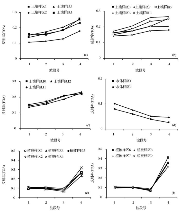
为了确定施密特正交化过程中用到的不同地物类型的典型样本,在所有的实验影像上选择了大量的干土壤、湿土壤、不同生长期的农作物、植被以及不同浑浊度的水体等样区,分别求出每个样区的平均光谱并分析其变化特征(图2)。可以发现,土壤的光谱差异相对较大,主要有3种变化特征(图2a~c),但总体上各波段的反射率都是逐步上升的;纯净水体的光谱特征相对较稳定,反射率从蓝波段到近红外波段稳步下降(图2d);生长期及成熟期的植被有着相似的光谱特征,但后者在近红外波段有更高的反射率,而在蓝光波段和红光波段则有更低的反射率。通过上述对不同地物光谱特征的分析,对所选样区进行筛选与合并(求均值),即可得到最能代表干土壤、湿土壤、成熟期植被和纯净水体等地物的最典型样本及其光谱特征。
图2 不同地物类型的光谱特征
(a)土壤光谱特征1;(b)土壤光谱特征2;(c)土壤光谱特征3;(d)水体光谱特征;(e)生长期植被光谱特征;(f)成熟期植被光谱特征
Fig.2 Spectral signature of different ground types
(a)Soil spectral signature 1;(b)Soil spectral signature 2;(c)Soil spectral signature 3;(d)Water spectral signature;(e)Spectral signature of growth vegetation;(f)Spectral signature of matured vegetation
从GF-1和Landsat 8同步的3幅影像(表1)中随机挑选了50万个样点做逐步回归,得到了GF-1影像4个波段表观反射率与Landsat 8 OLI缨帽变换的湿度分量之间的关系:
WetOLI=-0.233·ρ1+4.473·ρ2-3.886·ρ3-0.352·ρ4-0.078 (R2=0.79),(12)
式中:WetOLI是与GF-1同步的Landsat 8影像缨帽变换的湿度分量;ρ1,ρ2,ρ3,ρ4分别是GF-1影像蓝光、绿光、红光和近红外波段的表观反射率。空间向量a=(-0.233, 4.473, -3.886, -0.352)是由每个波段前的回归系数组成的,代表了湿度分量的方向向量,将其进行单位化(公式(6))得到的结果即是GF-1缨帽变换的湿度分量(A3)。固定湿度分量后,再用施密特正交化方法,结合前面得到的不同地物的典型样本光谱特征,可分别计算出缨帽变换的亮度和绿度分量,然后通过解方程组(公式(10))得到第4分量,即可获得GF-1 WFV2完整的缨帽变换系数(表2)。
表2 GF-1 WFV2缨帽变换系数
Table 2 TCT coefficient of GF-1 WFV2
| 缨帽变换分量 | 蓝光波段 | 绿光波段 | 红光波段 | 近红外波段 |
|---|---|---|---|---|
| 1. 亮度分量 | 0.2428 | 0.4347 | 0.4169 | 0.7604 |
| 2. 绿度分量 | -0.2637 | -0.4480 | -0.5584 | 0.6465 |
| 3. 湿度分量 | -0.0392 | 0.7530 | -0.6542 | -0.0593 |
| 4. 第4分量 | -0.9327 | 0.2082 | 0.2939 | 0.0177 |
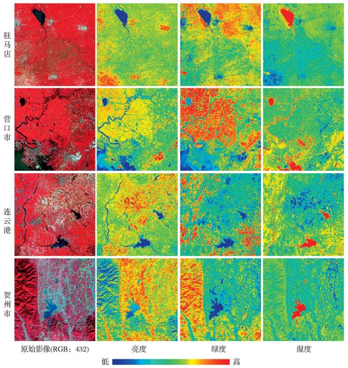
将表2中推导的缨帽变换系数应用到不同研究区的实验影像和验证影像上,获得了各幅影像的缨帽变换分量。图3给出了1幅试验影像和3幅验证影像的缨帽变换结果,从中可以看出各分量都有固定的变化规律,且不同区域的结果有很好的一致性。结合表2可以发现,缨帽变换的亮度分量是各波段反射率的加权和,占主导地位的是近红外波段,它反应了影像上不同地物的明暗程度,高亮度的土壤、建筑用地和亮红色的林地(标准假彩色显示)往往被突出显示,低亮度的植被(暗红色)和水体被抑制;绿度分量对植被敏感,代表植被的生长方向,主要受近红外与其他3个波段反射率的反差影响,植被在该分量上能够被突出显示;湿度分量对湿度敏感,主要受绿光和红光波段的反差影响,能够增强水体、植被和湿土壤并抑制建筑用地和干土壤;第4分量夹杂了大量的噪音,主要由噪音点构成(图3中未给出该分量图)。
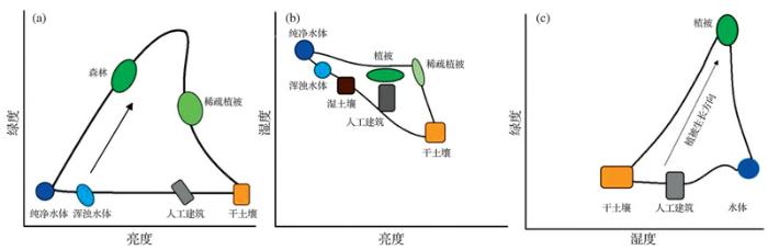
GF-1的缨帽变换结果代表了地物的特征空间,将其投影到平面上,可以更直观地考察地物在特征空间的分布特征,也是衡量缨帽变换结果的一个重要标志。缨帽变换不同分量之间构成的投影平面代表了不同的观测视角[12]:①亮度与绿度组成的投影平面是植被平面;②亮度与湿度组成的投影平面是土壤平面;③湿度和绿度组成的平面是植被和土壤2个投影平面之间的过渡带。对实验区GF-1 WFV2影像进行缨帽变换并将结果投影到不同的平面上,选取大量植被、水体、土壤、人工建筑等不同的地物类型并观察它们在不同投影平面上的分布特征。通过大量实验,发现它们在相应的投影平面上都有着独特的、相对固定的分布特征(图4)。图4a是亮度分量和绿度分量组成的植被平面,土壤线在底部基本上沿与坐标轴平行的方向分布,植被从土壤线上开始生长,随着生长期的变化,植被在亮度和绿度组成的特征空间中的分布基本上沿图中箭头所示方向变化。水体、植被、裸土、人工建筑等典型地物在其他不同投影平面上的分布见图4b,c。
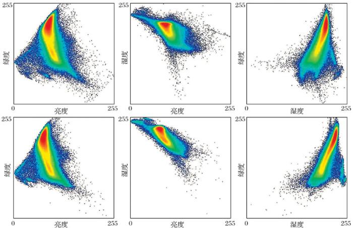
把所有验证影像缨帽变换的结果均投影到相应的平面上,发现尽管各影像的成像地区和时相不同,但地物在特征空间中不同投影平面上的分布都符合图4中的规律,这说明本文求出的缨帽变换系数合理地代表了地物的特征空间。限于篇幅,本文以其中1景有Landsat 8同步影像的区域为例,给出利用表2系数计算的GF-1 WFV2缨帽变换结果在不同投影平面上的分布特征(图5,第1行),并与已发表在国际期刊上并被广泛使用的Landsat 8缨帽变换结果在相应投影平面上的分布特征(图5,第2行)进行对比。图5中每1行的散点图从左到右依次是“亮度—绿度”、“亮度—湿度”和“湿度—绿度”。可以看出,尽管GF-1 WFV2和Landsat 8 OLI的传感器设置有很大不同,但其缨帽变换结果在对应投影平面上的分布特征仍然有相同的稳定模式,并且两者的分布模式有非常高的相似性,进一步说明了本文推导的缨帽变换系数的可靠性。
利用相关系数(R)和均方根误差(RMSE)指标,在2幅与Landsat 8同步的验证影像各分量影像上,采用等间距的方法随机抽取了12 000个样本点对表2中前3个分量进行检验。结果发现,尽管GF-1和Landsat 8影像在波段个数、波段设置和光谱响应上有很大不同,但其缨帽变换对应的各分量之间仍然有很好的相关性(表3),除了聊城市的湿度分量外,其他分量的相关性都大于0.85,甚至能达到0.9,而RMSE都低于0.1甚至低至0.05,说明了本文提出的GF-1 WFV2缨帽变换系数是适用和合理的。虽然2种传感器在波段个数、波段设置和光谱响应上有一定的不同,但经过合理的缨帽变换后,地物从光谱空间变换到特征空间,使得每个分量都代表特定地物的信息。例如,绿度分量集中反映了植被的信息,在任何传感器影像的缨帽变换绿度分量上,植被的绿度都会大于土壤的绿度。因此,尽管传感器的波段设置不同,但地物在特征空间(缨帽变换空间)中的分布规律却是相似的和相对稳定的。正是这种相似性和稳定性,使得GF-1和Landsat 8影像缨帽变换对应分量之间具有很好的相关性。
图3 原始影像及缨帽变换分量图(实验影像:驻马店;验证影像:营口市、连云港、贺州市)
Fig.3 The original images and their TCT components (Test image: Zhumadian; Validation image: Yingkou, Lianyungang and Hezhou)
图4 地物在不同投影平面上的理论分布特征
(a)植被平面;(b)土壤平面;(c)过渡带平面
Fig.4 Distribution characteristics of ground objects in different projection planes
(a)Plane of vegetation view;(b)Plane of soils view;(c)Plane of transition zone view
表3 GF-1和Landsat 8同步影像验证
Table 3 Validation using Synchronous images between GF-1 and Landsat 8
| 同步影像 | 缨帽变换分量 | 相关系数 | 均方根误差 |
|---|---|---|---|
| 亮度 | 0.8981 | 0.1079 | |
| 聊城市 | 绿度 | 0.8914 | 0.0956 |
| 湿度 | 0.8282 | 0.052 | |
| 亮度 | 0.9588 | 0.098 | |
| 连云港 | 绿度 | 0.9181 | 0.0671 |
| 湿度 | 0.8758 | 0.0598 |
通过对4波段传感器缨帽变换第3分量所解释的信息量占总信息量的百分比进行统计(表4),发现尽管前3个分量解释的信息量占总信息量的比例都大于98%,但第3分量所解释的信息量却都不超过2%,说明了地物在各波段的光谱信息投影到缨帽变换空间中主要沿第1分量和第2分量所组成的平面分布,只有少量数据分布在该平面外,这正是第3分量对前2个分量的方向变化非常敏感的原因。再加上GF-1 WFV传感器缺少对土壤湿度敏感的短波红外波段[13],给缨帽变换的第3个湿度分量系数的获取增加了不少难度。事实上,湿度分量对方向敏感性这一问题在其他缺乏短波红外波段的4波段传感器上一直都没能被很好地解决。Horne[20]虽然给出IKONOS的缨帽变换系数,却没有明确指出各分量所代表的含义;Yarbrough等[21]虽然给出了QuickBird 2的缨帽变换并指出第3分量为湿度分量,但是该分量对植被的湿度却有一定程度的低估;Sheng等[25]将CBERS-02B传感器缨帽变换的第3个分量定义为蓝度(Blueness),并未指出其与湿度之间的关系;Chen等[26]虽然将HJ-1 A/B传感器缨帽变换第3分量定义为湿度分量,但该分量与QuickBird 2的湿度分量一样,也会出现植被湿度被低估的问题。
表4 前2、3个分量能解释的信息变化量
Table 4 Total variance explained by the first 2 or 3 component
| 卫星传感器 | 前2个 分量/% | 前3个 分量/% | 第3 分量/% | 参考文献 |
|---|---|---|---|---|
| IKONOS | 98.3 | 99.8 | 1.5 | [20] |
| QuickBird 2 | 98.3 | 99.7 | 1.4 | [21] |
| CBERS-02B | / | 98.0 | / | [25] |
| HJ-1 A/B | 98.0 | 99.9 | 1.9 | [26] |
| GF-1 WFV2 | 97.3 | 98.9 | 1.6 | 本文 |
为了解决这一问题,本文实验后发现,在用施密特正交化方法推导出亮度分量和绿度分量后,无论是选择典型的水体样本然后与前2个分量正交化,还是通过与Landsat 8同步影像的湿度分量逐步回归然后再与前2个分量正交化,均不能得到理想的湿度分量。出现的问题主要表现为:①建筑用地的湿度常大于植被湿度;②植被湿度甚至大于水体的湿度;在大量的实验分析后,我们发现GF-1的亮度和绿度分量都具有一定的鲁棒性,对方向并不像湿度分量那样敏感。另外,从GF-1和Landsat-8同步影像的湿度分量回归结果来看,各波段反射率前的回归系数组成的4维空间向量能很好地代表湿度分量的方向,而从公式(13)计算的向量夹角可知,该方向向量与缨帽变换的前2个分量也接近于垂直正交。
因此,为了避免对回归系数组成的空间向量正交化所造成的以上2个问题,我们对常规的施密特正交化方法做了调整,直接把GF-1 WFV2的4个波段与Landsat 8湿度分量逐步回归的结果当作缨帽变换的湿度分量,仅对其进行单位化操作,然后再结合土壤和植被等典型样本的光谱特征,利用施密特正交化方法依次推导出亮度分量和绿度分量,从而很好地解决了4波段传感器缨帽变换中湿度分量对方向敏感的问题。
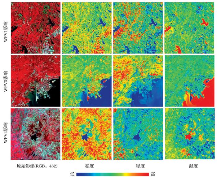
由于本文给出的缨帽变换系数只针对GF-1 WFV2传感器,对于这些系数在GF-1其他宽幅传感器WFV1,WFV3和WFV4上能否适用,本文也进行了实验检验。图6给出了将本文提出的系数应用到其他3个WFV传感器影像上得到的缨帽变换结果,第1行是WFV1传感器的原始影像和缨帽变换各分量图,从左到右依次是原始影像、亮度分量、绿度分量和湿度分量。第2、3行与第1行类似,分别是WFV3和WFV4传感器的原始影像和缨帽变换各分量图。从图6中可以看出,把表2中WFV2传感器的缨帽变换系数应用到其他WFV传感器影像上得到的各分量仍保持其固定的特征,并且与WFV2的结果有很高的一致性。
图5 缨帽变换结果在不同投影平面的分布特征 (0~255拉伸)
Fig.5 The tasseled cap distribution in different projection plane (Stretched between 0~255)
图6 GF-1其他3个WFV传感器缨帽变换结果
Fig.6 Tasseled cap transformation results of the other three WFV sensors in GF-1
利用表5中这3种传感器与WFV2传感器时相相近的影像,分别计算了各传感器的缨帽变换分量并统计它们与WFV2缨帽变换对应分量之间的相关系数(表6)。
表5 与WFV2传感器相近时相的影像对
Table 5 Images pairs between WFV2 and other sensors
| 地点 | WFV1 | WFV2 | WFV3 | WFV4 | 相差天数/d |
|---|---|---|---|---|---|
| 淮安 | 20160503 | 20160429 | / | / | 4 |
| 扬州 | 20160503 | 20160429 | / | / | 4 |
| 淮安 | / | 20160429 | 20160425 | / | 4 |
| 营口 | / | 20160919 | 20160920 | / | 1 |
| 淮安 | / | 20160429 | / | 20160430 | 1 |
| 聊城 | / | 20160504 | / | 20160517 | 13 |
表6 不同传感器之间缨帽变换的相关性统计
Table 6 Correlation statistics of tasseled cap transformation from different sensors
| 对比传感器 | 影像地区 | 亮度 | 绿度 | 湿度 | 第4分量 |
|---|---|---|---|---|---|
| 淮安 | 0.861 | 0.930 | 0.886 | 0.704 | |
| WFV1-WFV2 | 扬州 | 0.936 | 0.941 | 0.865 | 0.614 |
| 平均 | 0.899 | 0.936 | 0.876 | 0.659 | |
| 淮安 | 0.970 | 0.985 | 0.955 | 0.934 | |
| WFV3-WFV2 | 营口 | 0.908 | 0.887 | 0.893 | 0.791 |
| 平均 | 0.939 | 0.936 | 0.924 | 0.863 | |
| 淮安 | 0.810 | 0.909 | 0.853 | 0.706 | |
| WFV4-WFV2 | 聊城 | 0.751 | 0.907 | 0.854 | 0.665 |
| 平均 | 0.781 | 0.908 | 0.854 | 0.686 |
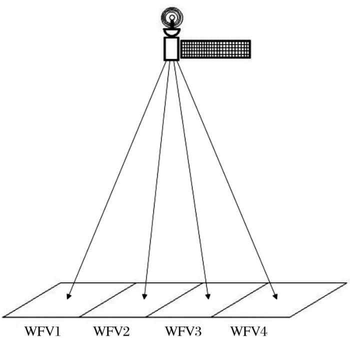
从表6中可以看出,WFV3与WFV2结果的相关性最高,前3个分量的平均相关性都超过了0.92。然后是WFV1和WFV2,它们前3个分量之间的相关性都高于0.85,其中绿度分量的相关性都大于0.9。相对而言,WFV4与WFV2之间的相关性最低,尽管绿度和湿度分量的相关性都大于0.85,但亮度分量的相关性却只有0.78。之所以出现这样的结果,是因为:①表5中的影像是非同步的(时间间隔相差1~13天),地表覆盖、大气条件在不同时相的影像上产生了一定的变化;②4个宽幅传感器之间的光谱响应有一定的差异,定标参数也有很大不同,导致不同传感器之间辐射信号并不是一致的;③4个传感器的观测角度不同(图7),由于WFV2和WFV3都是接近星下点(close-nadir)成像,对地物接近于垂直观测,两者观测方向差别不大。而WFV1和WFV4是远离星下点成像(off-nadir),对地物的观测角度与WFV2有很大的不同。受双向反射分布函数(Bidirectional Reflectance Distribution Function)的影响,不同观测方向的传感器接收到地物的反射信号也会有一定的差异,而且这种差异,在WFV1和WFV4传感器上表现得最为明显,这也是其与WFV2传感器缨帽变化结果的相关性差于WFV3的重要原因。
图7 GF-1 WFV传感器观测方向
Fig.7 Observation direction of different WFV sensors in GF-1
针对缺乏短波红外波段的GF-1 WFV2传感器,本文提出了一种改进的缨帽变换推导方法,调整了亮度分量、绿度分量和湿度分量的推导顺序,先用同步影像回归的方法确定湿度分量,然后再用施密特正交化方法推导亮度和绿度分量,从而很好地解决了缨帽变换系数推导时湿度分量对方向敏感性的问题。
把本文推导的缨帽变换系数应用在多幅不同地区的GF-1 WFV2影像上进行检验,发现不同分量的结果在各个区域的影像上都有很强的稳定性和一致性,说明本文提出的系数具有很好的适用性。通过与Landsat 8同步影像缨帽变换特征空间的对比后发现,尽管2种传感器波段设置及光谱响应能力不同,但却有着相似、稳定的特征空间。2种传感器对应的亮度分量和绿度分量之间的相关性能达到0.9,湿度分量之间相关性也都大于0.85,这都说明了本文提出的缨帽变换系数是合理的。
对GF-1上搭载的其他3个WFV传感器影像的研究结果表明,尽管本文的缨帽变换系数是针对WFV2传感器提出的,但同样可以拓展应用在WFV3和WFV1传感器上,其中以WFV3传感器效果为最好,各分量与WFV2结果的相关性都在0.9以上;其次是WFV1传感器,各分量与WFV2结果的相关性都大于0.85;而对于WFV4传感器来说,由于观测方向、扫描幅宽和空间分辨率等与WFV2均有较大差异,将本文提出的系数应用在该传感器影像上时会产生较大的不确定性,因此不建议在WFV4影像上使用本文提出的系数。
The authors have declared that no competing interests exist.
| [1] |
The tasselled cap—A graphic description of the spectral-temporal development of agricultural crops as seen by Landsat [C]// |
| [2] |
Monitoring desertification by remote sensing using the Tasselled Cap transform for long-term change detection [J]. |
| [3] |
Tasselled Cap transform for change detection in the drylands: Findings for SPOT and Landsat satellites with FOSS tools [C]// |
| [4] |
A comparative study of tasselled cap transformation of DMC and ETM+ images and their application in forest classification [J]. |
| [5] |
A remote sensing index for assessment of regional ecological changes [J].区域生态环境变化的遥感评价指数 [J].
基于遥感信息技术提出一个新型的遥感生态指数(RSEI),以快速监测与评价区域生态质量.该指数耦合了植被指数、湿度分量、地表温度和土壤指数等4个评价指标,分别代表了绿度、湿度、热度和干度等4大生态要素.与常用的多指标加权集成法不同的是,本研究提出用主成分变换来集成各个指标,各指标对RSEI的影响是根据其数据本身的性质来决定,而不是由人为的加权来决定.因此,指标的集成更为客观合理.将RSEI应用于福建长汀水土流失区,并与国家环境保护部《生态环境状况评价技术规范》中的生态指数EI的计算结果相比较,发现二者的结果具有可比性.不同的是,RSEI不仅可以作为一个量化指标,而且还可以对区域生态环境变化进行可视化、时空分析、建模和预测.因此,可弥补EI指数在这些方面的不足.
|
| [6] |
Derivation of vegetative variables from a landsat TM image for modelling soil erosion [J].
Abstract A study was carried out to assess the potential use of satellite thematic mapper (TM) images to produce maps of vegetation-related variables for erosion modelling. In a Mediterranean study area in southern France the (semi-)natural vegetation was described at 33 field plots using four quantitative methods: the Fosberg structural classification system, the cover and management factor of the Universal Soil Loss Equation, the leaf area index and the total percentage cover. After radiometric correction of the image, the spectral TM bands were processed following three different methods. Each method aimed at combining the data of the six spectral TM bands into a single band in such a way that the resulting image displayed optimal information on green vegetation cover. The algorithms used comprise the normalized difference vegetation index, the conventional 鈥榯asselled cap鈥 transformation and a locally tuned tasselled cap transformation. Only slight differences were found between the different methods to calculate spectral vegetation indices for this particular case. Furthermore, the correlations between the field variables and image-derived spectral indices are generally small. The largest correlations were found for the normalized vegetation index and the leaf area index ( r + 0路71) and for the normalized vegetation index and Fosberg's structural vegetation classes ( r + 0路76). However, Fosberg's method results in very general classes, which are of little use for soil erosion models. Furthermore, the spectral indices appeared to be sensitive for the vitality of the vegetation. Consequently, an area covered by a sensed, senescent vegetation will not yield a large value for the spectral index, but its soil is protected against splash erosion. This might lead to a misinterpretation of the soil protective cover when satellite images are used. A final conclusion is that a balance has to be found between the more accurate, but time-consuming field surveys to gather information on erosion-controlling factors and a certain loss of accuracy associated with the use of quick and easy remote sensing methods.
|
| [7] |
An efficient protocol to process landsat images for change detection with tasselled cap transformation [J]. |
| [8] |
MODIS tasselled cap: Land cover characteristics expressed through transformed MODIS data [J].
The tasselled cap concept is extended to Moderate Resolution Imaging Spectroradiometer (MODIS) Nadir BRDF‐Adjusted Reflectance (NBAR, MOD43) data. The transformation is based on a rigid rotation of principal component axes (PCAs) derived from a global sample spanning one full year of NBAR 16‐day composites. To provide a standard for MODIS tasselled cap axes, we recommend an orientation in MODIS spectral band space as similar as possible to the orientation of the Landsat Thematic Mapper (TM) tasselled cap axes. To achieve this we first transformed our global sample of MODIS NBAR reflectance values to TM tasselled cap values using the existing TM transformation, then used an existing algorithm (Procrustes) to compute the transformation that minimizes the mean square difference between the TM transformed NBAR values and NBAR PCA values. This transformation can then be used as a standard to rotate the MODIS NBAR PCA axes into a new MODIS Kauth–Thomas (KT) orientation. Global land cover patterns in tasselled cap space are demonstrated graphically by linking the global sample with several other products, including the MODIS Land Cover product (MOD12) and the MODIS Vegetation Continuous Fields product (MOD44). Patterns seen at this global scale agree with previous explorations of TM tasselled cap space, but are shown here in greater detail with a globally representative sample. Temporal trends of eight smaller‐scale BigFoot Project (www.fsl.orst.edu/larse/bigfoot) sites were also examined, confirming the spectral shifts in tasselled cap space related to phenology.
|
| [9] |
Estimating soil salinity in the Yellow River Delta, Eastern China—An integrated approach using spectral and terrain indices with the generalized additive model [J]. |
| [10] |
Multivariate correlations between imagery and field measurements across scales: Comparing pixel aggregation and image segmentation [J]. |
| [11] |
Comparison of quality evaluation methods for image fusion of farmland remote sensing [J].农地遥感图像融合质量评价方法比较 [J].
为更加客观公正地比较融合结果、评估融合算法及优化融合过程,该文在分析主要遥感图像融合质量评价方法的基础上,将定量评价指标分为三类:评价图像亮度信息的指标、评价空间信息保持能力的指标和评价光谱信息保持能力的指标。最后,通过仿真试验,以光学遥感图像融合为例,验证了4种常用的像素级融合算法的适用性和有效性。IHS变换法扭曲了源图像的光谱特性,容易产生光谱退化;Wavelet变换法在光谱特性保持方面具有优势,但容易出现分块效应和模糊现象;PCA变换法较多地保留了源图像的细节纹理和结构特征,但会失去源图像的部分物理特性;缨帽变换法融合结果地物边缘清晰,但对细微光谱信息的保持能力较弱。研究表明,这3类指标可以作为遥感图像融合的客观效果评价准则,并为融合结果的后续应用提供借鉴意义。
|
| [12] |
A physically-based transformation of thematic mapper data—The TM tasseled cap [J]. |
| [13] |
Application of the Tasseled Cap concept to simulated thematic mapper data [J].
ABSTRACT Thematic Mapper signal counts in the six reflective bands (i.e., excluding the thermal band) are simulated using field and laboratory spectrometer measurements of a variety of crops, crop conditions, and soil types. The Dave atmospheric model and prelaunch sensor characteristics comprise the other components of the simulation. The simulated data are found to occupy essentially three dimensions, two of which are equivalent to the MSS Tasseled Cap Greennes and Brightness features, and a third which is substantially influenced by the mid-infrared bands of the TM. This new dimension is primarily related to soil characteristics, including soil moisture. The nature and characteristics of each dimension are discussed, as are some of the expected information gains (over MSS data) resulting from the additional dimensionality of the data.
|
| [14] |
Derivation of a tasselled cap transformation based on Landsat 7 at-satellite reflectance [J].
A new tasselled cap transformation based on Landsat 7 at-satellite reflectance was developed. This transformation is most appropriate for regional applications where atmospheric correction is not feasible. The brightness, greenness and wetness of the derived transformation collectively explained over 97% of the spectral variance of the individual scenes used in this study.
|
| [15] |
Derivation of a tasselled cap transformation based on Landsat 8 at-satellite reflectance [J].
The tasselled cap transformation (TCT) is a useful tool for compressing spectral data into a few bands associated with physical scene characteristics with minimal information loss. TCT was originally evolved from the Landsat multi-spectral scanner (MSS) launched in 1972 and is widely adapted to modern sensors. In this study, we derived the TCT coefficients for the newly launched (2013) operational land imager (OLI) sensor on-board Landsat 8 for at-satellite reflectance. A newly developed standardized mechanism was used to transform the principal component analysis (PCA)-based rotated axes through Procrustes rotation (PR) conformation according to the Landsat thematic mapper (TM)-based tasselled cap space. Firstly, OLI data were transformed into TM TCT space directly and considered as a dummy target. Then, PCA was applied on the original scene. Finally, PR was applied to get the transformation results in the best conformation to the target image. New coefficients were analysed in detail to confirm Landsat 8-based TCT as a continuity of the original tasselled cap idea. Results show that newly derived set of coefficients for Landsat OLI is in continuation of its predecessors and hence provide data continuity through TCT since 1972 for remote sensing of surface features such as vegetation, albedo and water. The newly derived TCT for OLI will also be very useful for studying biomass estimation and primary production for future studies.
|
| [16] |
A tasseled cap transformation for Landsat 8 OLI TOA reflectance images [C]// |
| [17] |
Comparison of tasselled cap transformations based on the selective bands of Landsat 8 OLI TOA reflectance images [J]. |
| [18] |
Study of derivation of tasseled cap transformation for Landsat 8 OLI images [J].Landsat8陆地成像仪影像的缨帽变换推导 [J]. |
| [19] |
Using at-sensor radiance and reflectance tasseled cap transforms applied to change detection for the ASTER sensor [J]. |
| [20] |
A tasseled cap transformation for IKONOS images [C]// |
| [21] |
QuickBird 2 tasseled cap transform coefficients: A comparison of derivation methods [C]// |
| [22] |
Evaluation of SPOT imagery for monitoring irrigated lands [C]// |
| [23] |
Determination of 'tasseled cap' transformation parameters for images obtained by the SPOT satellite [C]// |
| [24] |
Orthogonal transformation of segmented SPOT5 images [J].
Brightness, Greenness, and Wetness Tasselled Cap parameters were derived for the SPOTS sensor. Their robustness through space and time and their discrimination power in land-cover classes was investigated. Four images were acquired from March and September 2003, and in July and November 2004 over Germany. A fifth SPOTS image was acquired from Cameroon, West Africa in January 2003. The Tasselled Cap parameters were extracted with the Gram-Schmidt orthogonalization technique for each image independently. One set of combined parameters was created for Germany using samples from the four SPOTS images simultaneously. Each SPOTS image was transformed into Brightness, Greenness, and Wetness with their own with the combined and the July parameters. Spearman's Rho correlation analysis was carried out between the Tasselled Cap counterparts acquired with the various parameters. Brightness exhibited nearly perfect correlations between the images in Germany; in Cameroon however, the images were inconsistent. Greenness and Wetness displayed a difference of up to 35 percent in November in Germany. The Wetness counterparts in Cameroon exhibited a 7 percent difference. Canonical discrimination analysis revealed that the components from July had the highest discrimination power and that Greenness expressed the highest association to the first canonical axis in all images. In March, July, and November, Brightness was the second most important Tasselled Cap component, in September the Wetness and in Cameroon the Greenness. These results indicate that the Tasselled Cap components are not stable between different seasons and geographical locations. They can be successfully used for land-cover discrimination if the images are transformed with parameters appropriate to the investigated season respective biogeographical zone.
|
| [25] |
A tasseled cap transformation for CBERS-02B CCD data [J]. |
| [26] |
Tasseled cap transformation for HJ-1A/B charge coupled device images [J].
At-satellite reflectance based tasseled cap parameters were extracted from HJ-1A/B satellite imagery, the charge coupled device (CCD) data of the Chinese environmental satellites that were launched on September 6, 2008. Sixteen scenes selected from the four sensors (HJ 1A CCD1, HJ 1A CCD2, HJ 1B CCD1, HJ 1B CCD2), respectively were used. The objectives are evaluating the consistency of the tasseled cap parameters for four sensors and proposing combined tasseled cap parameters for all four HJ-1A/B CCD. The results indicated that the direction of corresponding tasseled cap vectors of four sensors were almost the same. Then a combined at-satellite reflectance-based tasseled cap transformation was developed based on eight HJ-1A/B CCD scenes representing a variety of landscapes of China in both leaf-on and leaf-off seasons. Extraction combines the principle component transform with Gram-Schmidt Orthogonalization (GSO) process. The accurate brightness was obtained with the help of the first principal component eigenvector, and then greenness and wetness. The fourth one was obtained by the GSO. The first two dimensions (the brightness and the greenness) typically capture over 98%, and the brightness, greenness, and wetness account for over 99.9% of the total spectral variance. The fourth one occupies a very low proportion.
|
| [27] |
Summary of current radiometric calibration coefficients for Landsat MSS, TM, ETM+, and EO-1 ALI sensors [J]. |
| [28] |
Image-based normalization technique used for Landsat TM/ETM+ imagery [J].
The development of the image-based normalization technique used for Landsat Thematic Mapper/Enhanced Thematic Mapper Plus imagery is reviewed.The techniques perform radiometric calibration by converting the digital number of the Landsat imagery to at-satellite radiance and then to at-satellite reflectance using data normalization method.The validation case in this study shows that the illumination difference between the tested multitemporal Landsat TM images can be considerably reduced to one-third of that of the original DN-based image through the normalization technique.
|
| [29] |
Retrieval of reflectance and land surface temperature of the newly-launched Landsat 8 satellite [J]. |
| [30] |
Spectral indices in n-space [J].
Linear combinations of spectral bands form physically significant indices in space. The 2-dimensional (2-D) perpendicular vegetation index () of Richardson and Wiegand and the 4-D tasseled cap of Kauth and Thomas are special cases of indices. A procedure for calculating the coefficients of indices is described. Spectra from 12 and two soil (wet and dry) plots were multiplied point by point (at 1-nm intervals) by response functions representing five satellite sensors. Reflectance values were obtained for each band for each sensor (atmospheric effects and sensor characteristics such as noise, resolution, and calibration, were not considered). indices were calculated for various band combination for the several sensors and their dynamic range for a 0鈥100% change in vegetation was compared. A 6-D vegetation index (greenness) calculated using six of the thematic mapper bands had the greatest dynamic range, followed closely by two 5-D and one 4-D greenness from the same sensor. The 2-D greenness using bands 4 (near-IR) and 7 (mid-IR) of the thematic mapper had a greater dynamic range than any band combination of the other four satellite sensors. The 4-D greenness of the Landsat-4 MSS and the 3-D index of the SPOT HRV were similar. The 2-D indices from the AVHRR sensors on NOAA-6 and NOAA-7 changed less with vegetation changes than did the other three.
|

/
| 〈 |
|
〉 |
