基于地质力学方法的低渗透砂岩储层构造裂缝预测研究
[冯建伟 , 任启强, 徐珂]
, 任启强, 徐珂]
|
|


作者简介:冯建伟(1979-),男,山东临朐人, 副教授,主要从事构造地质学和地质力学研究.E-mail:Linqu_fengjw@126.com
目前,研究并搞清构造裂缝的形成时间、位置、产状、规模及分布密度对于低渗透、超低渗透砂岩储层的勘探开发至关重要,但具有很大难度。基于应变能理论建立一套综合地质力学模型以定量预测裂缝参数及分布,如裂缝线密度和体密度等。首先,在岩石力学实验的基础上将脆性储层中由构造应力引起的总能量划分为裂缝表面能、摩擦耗能和残余应变能3种类型,其中前两者即为与裂缝产生相关的能量,并以此为桥梁推导建立应力—应变和裂缝参数之间的关系模型。其次基于地震解释结果建立复杂构造区含断层的古地质模型、岩石力学实验、测井解释,通过动静校正的方法获得砂岩、泥岩的强度参数,从而建立地质力学模型。最终,进行古应力场数值模拟计算裂缝参数三维展布特征,并以实际井点数据进行验证。结果表明地质力学模型法不同于一般的几何分析方法,具有较高的可靠性和适用性,能够预测不同构造运动阶段的裂缝参数分布,并能够进行三维空间显示;裂缝的充填程度不仅影响着裂缝开度,也在很大程度上影响着低渗透砂岩储层的渗流特征,这对于进一步实现现今裂缝开度的定量预测以及储层数值模拟具有重要意义。
First author:Feng Jianwei(1979-),male,Linqu County, Shandong Province,Associate professor. Research areas include structural geology and geomechanics.E-mail:Linqu_fengjw@126.com
Understanding and interpreting the timing, location, orientation, and intensity of natural fractures within a geological structure are commonly important to both exploration and production planning activities of low-porosity and low-permeability carbonate reservoirs. In this study, we explore the application of comprehensive geomechanical methods to quantitatively characterize the fracture parameters based on Strain Energy Density Theory, such as linear fracture density and volume fracture density. This study approach is based on the idea that energy generated by tectonic stress on brittle sandstone,which can be distinguished fracture surface energy, friction energy dissipation and residual strain energy and natural fractures can be interpreted or inferred from geomechanical-model-derived strains. For this analysis, we model an extension and compression compound fault block developed in a mechanically stratified sandstone and shale sequence because mechanics experimental data and drilling data exist that can be directly compared with model results.However, the results show that the approach and our study conclusion are independent of the specified structural geometry, which can correlate fracture parameters in different stages with different tectonic activities, and finally build and visualize fracture networks in sandstone. The presence or absence of filling minerals in fractures is shown to strongly control the destruction and transformation of low-permeability sandstone, and this control possesses crucial implications for interpreting fracture aperture and reservoir flow simulation.
Natural fractures impact the performance of many reservoirs, including some of the carbonate reservoirs, tight sand reservoirs and low-permeability reservoirs in the world[1~4]. Understanding and interpreting where and when fractures develop within a geological structure along with their orientation and intensity are important to both exploration and production planning activities. Controls on fracture development include proximity to faults, position on folds, stress intensity, lithology and their combination and layer thickness[5~11]. Many studies have found that fractures often were developed around fault zone and anticlinal core, and fracture spacing is positively correlated with regional stress intensity[12~14], whereas other researchers suggest that lithology and their combination may be more significant than regional stress[15~18]. Someone even found that the natural fracture networks tend to be heterogeneous and messy near formation interfaces, when the stratum consist of hard and soft rocks, in which fractures are clustered in swarms and irregularly distributed[7].
As practiced in fractured reservoir exploration and production, fracture prediction is commonly based on geometric and/or kinematic models such as analyses of fault-related folds and old curvature or seismic techniques or logging techniques to acquire interwell fracture networks and the attributes, but far less with geomechanical modeling[19~23]. However, numerical geomechanical modeling such as finite element, boundary element and discrete element can provide powerful tools for simulating the spatial and temporal development of geological structures[4, 24~30]. This paper have found the application of finite-element-based geomechanical models which have excellent potential for understanding and interpreting natural fractures in geologic structures. Finite element modeling allows complex geometries (e.g., faults and mechanical stratigraphy) to be combined with realistic material models to produce physically realistic and mechanically rigorous forward models. The basic premise of this approach is that the geomechanical-model-derived permanent strains can be acquired in terms of fracture characteristics (i.e., location, orientation, and intensity). And the kinematic history is captured by this approach and further permits tracking the spatial and temporal evolution of stress and strain in the eformed rocks or beddings[4, 22, 30, 31].
Since the 1960s, many studies have been published by the mechanical methods of structural movement on the generation of fractures, including rock failure criterion and strain energy density. Price[32] proposed that the fracture intensity had fine positive correlation with elastic strain energy in rocks based on laboratory modeling experiments and tests, and then he described a method using the Coulomb failure criterion to explain the critical factors in triggering earth-quakes along a proximal fault. Wen et al.[33] and Song[34] successfully used tensional failure criterion and shear failure criterion to calculate rock cracking index in predicting fractures development zone and dominant orientation. Wang et al.[35], Zhou et al.[36]and Tan et al.[37]put forward a quasi-binary method combing failure degree value and energy degree value to quantitatively characterize fracture density based on the theory formation with high strain energy possessing more fractures than rocks with low strain energy, and the calculated and practical results are in good agreement. Dai et al.[38] tried to establish a series of formulas between stress-strain and fracture volume density based on certain assumption that paleostress field generates cracking and the current stress field only induces some minor changes in fractures size instead of producing new cracks, simultaneously considering filling degree in fractures.
Commonly, the fracture prediction includes fracture identification, available failure criterion selection, and spatial parameters characterization. Although previous experimental and numerical studies provide a general understanding of the failure mode, propagation mechanism of cracks in rock mass, however, so far the quantitative prediction of fracture parameter has not been resolved, the energy distribution relationship at the course of deformation has not been studied comprehensively, and the quantitative influence of current stress field on paleo fracture system has not been confirmed. This paper provides a comprehensive geomechanical approach by describing full-scale fracture formation mechanisms in cores and establishing quantitative relations between stress-strain and fracture parameters to predict the spatial distribution of stress perturbations and the likelihood of fracture generation at the base of abundant rock mechanical tests.
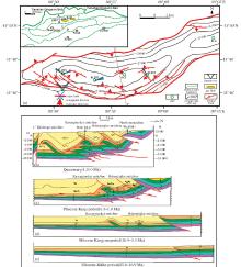
The Kuqa Depression is located at the northern margin of the Tarim Basin between the South Tianshan Orogenic Belt and the Northern Tarim Uplift to the south (Fig.1). Thrust faults and related folds widely developed in the Kuqa Depression during the Cenozoic time structures are dominated by, and laterally, the Kuqa Depression can be divided into three structural belts and two sags, which are the northern monocline belt, Kelasu structural belt, Baicheng sag, Kuqa depression, and Qiulitage structural belt from north to south[40, 41] (Fig.1). Since the late Cretaceous the Kuqa Depression had experienced a complex evolutionary history as a consequence of the northward Indian sub-continent and southward thrusting of the South Tianshan, which is recognized as one of the major Cenozoic depocenters along the margin of the Tarim Basin[42~44]. Kela-2 gas field is situated in the upper wall of Kelasu tectonic belt and south of Kela fault, displaying brachy anticline with structure amplitude less than 500 m, the top of which was cross-cut by a series of subsidiary faults striking EW to become complicated, with dip of southern wing ranging from 19° to 23° and northern wing ranging from 16° to 20° (Fig.1).Intervals of fracture in Kela-2 gas field are consisting of Cretaceous delta front rocks(the Lower Bashijiqike Formation, K1bs), which is dominated by fine sandstone, siltstone and mudstone together with limited sandy conglomerate. A total thickness of these beds can reach 270 m in the study area and are further divided into three members according to lithological cycles and interbeds. The porosity Bashijiqike reservoir ranges from 2%~7% through core test and permeability lies in range of 0.05× 10⁻³~0.50× 10⁻³ μ m2, however the fracture permeability can reach 1.00× 10⁻³~10.00× 10⁻³ μ m2. Finally, all the above evidences prove that the Kela-2 gas field belongs to typical ultra-deep low-porosity and low-permeability tight sandstone reservoir.
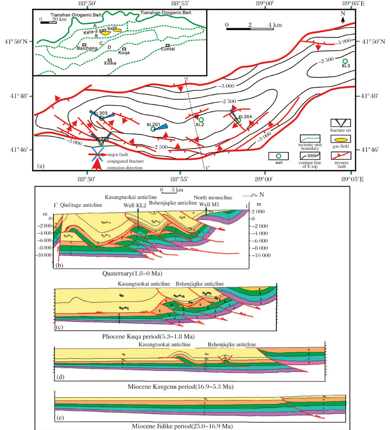 | Fig.1 Structural simplified map of the Kuqa Depression within the Tarim Basin, China and Schematic representation of the tectonic history at Kelasu Anticline[39] (a) Sets(blue) of fractures in Well KL202 and Well KL203 are parallel or perpendicular to faults in the west, and sets(blue) of fractures in Well KL201 are skewed to faults in the central, fractures in Well KL204 are parallel to accommodation fault in the east; (b) Present-day structure; (c) Removal of displacement along the southern reverse faults; (d) Geometry of restored horizons to the top of the Kangcun Formation; (e)Geometry of restored horizons to the top of the Jidike Formation |
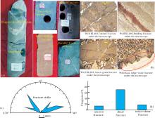
The most frequently encountered fractures in thereservoir of the area are planar discontinuities that are sub-perpendicular to the bedding, which can be divided into three basic types, tension fracture type, tenso-shear fracture type and shear fracture type. Each type is also characterized by a distinct fracture shape, such as the shear fracture always has more straight fracture plane and longer extended distance than those two types, in most cases, which can cut through rock grains, however the extension fracture exposes dendritic structure and frequently bypasses rock grains with a relatively shorter distance, wherever these types are observable by drill core and microscope(Fig.2a, b).Based on the orientation, the fractures present in the Bashijiqike Formation can be subdivided into four distinct, mutual abutting fracture sets oriented NW-SE (set I), NNW-SSE(set II), NE-SW (set III) and NNE-SSW (set IV) (Fig.1, Fig.2). On minor faults associated with southern major fault, several kinematic indicators show a sinistral strike-slip motion along this fault (Fig.1). Fault nearby Well KL204 was charac- terized by an abnormal strike NW330° and nearly vertical plane, and was limited by two NNE-SSW striking faults, which indicates obvious internal slipping and accommodative movement in strong structural activity period.
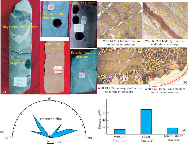 | Fig.2 Characteristic of structural fractures in Kela-2 area, Kuqa Depression (a) Examples of representative fracture samples from different drill cores with diameter ca. 10 cm, where tension fracture has irregular shape and extend after bypassing rock grains, however shear fracture has perfectly straight fracture plane and directly cut through rock grains, neutrally the character of tenso-shear fracture lies between both. (b) Photos of different types micro-fractures in thin sections. (c) Orientation rose diagram of fracture lineaments in Bashijiqike reservoir (207 data points).(d) Histogram of fracture mechanical property. Shear fractures occupied the highest proportion than tenso-shear fractures and tension fractures (207 data points) |
Fractures of Set II inWell KL203 are parallel to Kela-2 fold axial plane in the west, the dip angles, visible on the cores (Fig.2a), are sub-perpendicular to the folded bedding, which can accommodate the bed lengthening due to fold curvature. Fractures of Set IV in Well KL203 and Well KL201 in the west and middle part skew to the fold axis with a low-angle 25° , are still sorted to tension fractures with Set II caused by outer-arc tension at the folding stage of Pliocene Kuqa period. However, fractures of Set I and Set III in Well KL202 and Well KL204 are characterized by an irregular spatial distribution (localized swarms) and a scattering in strike, in contrast the two previous sets. This scattering is observed in particular where the fold curvature variates and minor faults develop (Fig.1), which indicate that the regional compressional event and local shear event have generated conjugated fractures, but the former is mainly composed of net-shaped conjugated fractures and with length and vertical extent often greater than 10 m, is characteristic of systematic joints as defined by Zhao[39].On the basis of the previously detailed observations and tectonic history, we consider two major stages for the fracture formation and folding development from the beginning of the Himalayan orogeny. Fig.1a shows the orientations of the principal stress axes, which obtained from the inversion of kinematic indicators (slicken lines and conjugated fractures) observed and measured on minor faults associated with boundary major fault, they are nearly SN-trending compressional stress in the region before the Basehnjiqike formation deformation and SN-trending tensional stress on the Kela-2 reservoir folding[45].
In this paper, the Uniaxial and Triaxial Mechanics Instrument(ITEM:TAWA-2000), which is a hybrid loading equipment under maximum axial pressure 2 000 KN and maximum confining pressure 140 MPa for uniaxial compression test and triaxial compression test, was used to simulate the failure process. The rock samples cored at different directions with respect to the plane of initial fracture coming from the third section of Bashenjiqike Formation (K1bs) Kela-2 area in Kuqa depression. Each sample was prepared by ISRM suggested method (ISRM, 2007) with diameter of 50 mm and length of 100 mm, with ends grounded to be flat to 0.01 mm and less than 0.2 mm, and the vertical deviation was less than 0.25° . Triaxial tests were carried out by multi-stage loading method, and the loading rate was set to 0.01 mm/s. In loading course the confining pressure was set to eleven stages with interval of 5 MPa:0 MPa, 5 MPa, 10 MPa, 15 MPa, 20 MPa, manually as the axial pressure increases where at all times axial loads exceed confining pressure by no more than one tenth of the rock UCS until peak stress reached[46]. In this study, the mechanical parameters (e.g., σ t, σ c, τ s, E, G, μ , C0 and φ ) of low-permeability sandstone were acquired (Table 1, Table2).
| Table 1 Experimental datasets from uniaxial compressive tests |
After a series of tests, rock strength and mechanical properties were documented in Table 1 and Table 2 by uniaxial compressive tests, triaxial compressive tests and splitting tests etc. Where σ t is the tensile strength of intact rock, τ s is the shear strength, σ c is the uniaxial compressive strength, E is the Young’ s modulus or elastic modulus, G is the shear modulus, μ is the poisson’ s ratio, C0 is the cohesive strength of rock, φ is the friction angle of rock. According to the obtained rock properties listed in Table 1, the failure mode are categorized by σ c, σ t, τ s, E, G and μ as different anisotropy rocks[47].It can be concluded that the calcareous siltstone has stronger brittleness than other sandstones, such as fine sandstone, siltstone, argillaceous sandstone, etc.Table 2 shows the variation of triaxial compressive strength and friction angle of the fine sandstone and siltstone with respect to different confining pressures. It should be noted that the maximum peak strength will be obtained when the confining load is close to real underground conditions(approximately 5 MPa).
| Table 2 Experimental datasets from triaxial compressive tests |
Fig.1 compares the mechanical properties with failure mode of different sandstone in study area according to the above mentioned. Three failure modes were identied: Tension failure, shear failure and mixed failure (tenso-shear fracture). Accordingly the extensional fracture criteria and shear fracture criteria should be taken together to explain the failure behavior of intact rock masses[33]. Generally, in numerical modeling of tectonic stress field, Griffith Criterion is utilized for the calculation of extensional fracture, and Coulumb-Mohr Criteria is preferred for orientation of shear fracture[48, 49]. As a matter of fact, under condition of high confining pressure, high temperature and slow loading ratio, a kind of shear fracture with angle less than 45° oblique to the pressing direction will occur. On the contrary, under rapid loading ratio, dilated breaking will occur parallel to compression direction, which belongs to typical brittle failure mode[50].
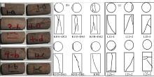
As depicted in Fig.3, variation of failure forms and combination show a transitional trend with various confining pressure. There are actually many reasons that explain differences between failure modes obtained for criterions such as stresses, cohesion, friction and mineralogy of rocks. Hence, cohesive strength, C0 and friction angle, φ of siltstone and finestone were determined from linear portion of Mohr envelopes at θ =24.5° and θ =19.09° as presented in Table 2. Among the samples, there appeared a large number of fissures and fractures, consisting of types of tension, compression and shear, such as sample K101-DC3, K101-DA4 and K101-DA2 performed as tension-shear opening fractures, sample K103-DA3, K101-DB3 and K105 performed as shear fracture, with some tensile characteristics. Among them, fracture trace in sample K101-DB3 is characterized by a series of tensile micro-cracks to form and propagate into macroscopic shear zone with angle of rupture less than 45° , just coinciding with the Mohr-Coulomb theory. However, Jaeger and Hoek and Brown’ s works are of importance that they thought the failure criterion should be modi-ed to take into account the anisotropy of strength properties. Rupture shapes through triaxial compression tests in Fig.3c, such as sample L12-1, L12-2 and L12-3 respectively with confining pressure 5 MPa, 10 MPa and 15 MPa, and sample L25-1, L25-2and L25-3 respectively with confining pressure 5 MPa, 10 MPa and 20 MPa, etc., are obviously different from that of unaxial samples. As a result, it can be concluded that the fracture mechanical property is mostly influenced by state of stress and certain confining pressure, i.e., along with the increasing confining pressure, the shear action becomes stronger, and the angle of rupture increases(Fig.3c).
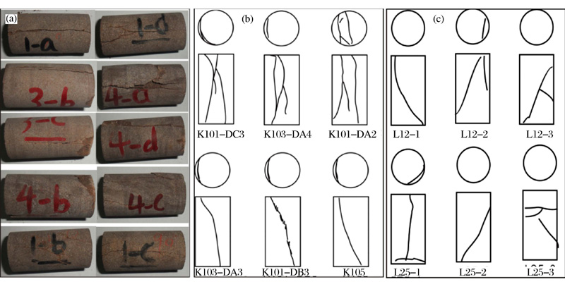 | Fig.3 Results of different rocks after mechanical experiments with different confining pressure (a) Rock failure modes of uniaxial compressive tests. (b) Rock failure modes of triaxial compression tests. (c)Standard rock samples coming from drill cores used for texts |
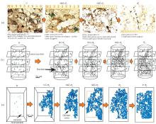
Generally, thedifferences between mechanical parameters or properties are mainly influenced by multiple factors including rock composition, confining pressure, pore pressure, temperature, fluid media, loading ratio, etc. For this study, predecessors in this field have already done a lot of interesting researches, and achieved fruitful results. On the basis of the above experiments, we can change the next experiment scheme as follows: To select core samples coming from Kela-2 gas field in Kuqa Depression with similar lithology and mechanical properties, including some initial microcracks or weakness planes to simulate the failure process. To acquire complete stress-strain curves and σ c(peak strength) in strength tests under uniaxial stress, the CT MPR and microscopic thin section observations were carried out to record the fracture evolution process at different loading stage, i.e.σ c 10% σ c 20%, σ c 30%, ……, σ c 80%, σ c 95% with steady rate(0.01 mm/s). After loading, rock samples were taken out and consolidated with glue, either to be scanned on equipment— CD-600BX or observed on level thin section and vertical thin section under a high-powered microscope(Fig.4). Finally, based on a series of stress-strain curves, the strain energy density and fractures density of low-permeability sandstone were calculated and described in detail to set up certain relationship between stress and fracture parameters.
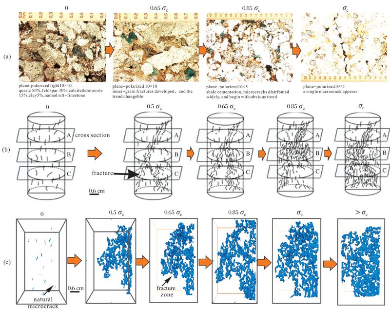 | Fig.4 Evolution diagram of microcracks in low-permeability sandstone under uniaxial cyclic compression tests (a) Thin slices of microcracks and macrocracks obtained parallel to the cross-section of rock samples under plane polarized light.(b)Overview of microcracks statistics by slice A, B, C in low-permeability sandstone after compression test.(c) Inner cracks are finely scanned with CT scanner (precision less than 10um) at different loading stages(0, 0.5 σ c, 0.65 σ c, 0.85 σ c, σ c and > σ c) and finally 3D-crack images are reconstructed |
Based on mechanical tests of medium grain marble, granite and aplite, Brace et al.[51]divided the brittle deformation course into four stages: Compaction, elastic deformation, dilatation and failure. According to axial and radial strain curves, at first, most microcracks in rocks propagate along weaknesses spots sequentially, when reach the region of one-third and two-thirds of uniaxial compression strength, the rocks dilate obviously and produce a large number of cracks. Therefore, the macroscopic behavior of rock is generally controlled by number of microcracks and rock properties.
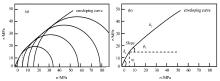
Recently, a lot of arguments for cracking mode under tensile stress appeared, some thought that shear fractures only formed under deep triaxial stress conditions, and extensional fractures only form under shallow tensile stress conditions. Through many experiments, Dai et al.[52] and Omid et al.[46] discussed the possible conditions for shear fractures with tensile stress existing, which indicated that tension criterion should be preferred to determine whether extensional fracture occurred firstly. If no fracture took place, then Mohr-Coulomb criterion would be used to determine whether shear fracture occurred, was known as a kind of combined tension-shear failure criterion. Firstly, an enveloping curve was extracted from a series of Mohr circles on base of experimental results, then two-step Mohr-Coulomb curve is drew out[53], as shown in Fig.5.
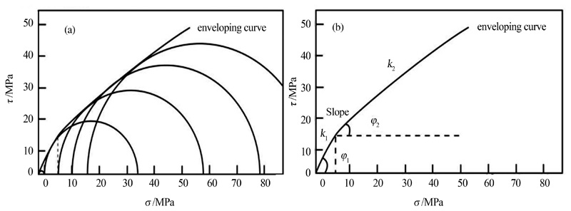 | Fig.5 Mohr enveloping curve of low-permeability sandstone (a) and two-step Mohr-Coulomb curve in study area(b) extracted from triaxial compression tests |
Here, φ 1, φ 2 respectively is internal frictional angle under different confining pressure, k1, k2 respectively is the straight slope in curve, and σ 0=5 MPa is cut-off value of confining pressure. It can be concluded as follows:Fig.5 implies the strong relationship between confining pressure and failure modes, i.e. when the confining pressure is less than a value, φ is quite large, and θ =45° -φ /2 is relatively small, extensional fracture is popular. When confining pressure is relatively large, failure mode will transform to shear fracture or compresso-shear fracture. The detailed relative equations as follows:
If 0< σ 3≤ σ 0=5 MPa,
φ =φ 1=51.83° (angle of rupture)
θ =θ 1=45° -φ /2=19.09° (1)
If σ 3> σ 0=5 MPa, φ =φ 2=41° (angle of rupture)
θ =θ 2=45° -φ /2=24.5° (2)
Thus, it is not difficult to find that under compression tress state, the two-step Mohr-Coulomb criterion is preferred for the low-permeability sandstone[47, 50]. However, under tension stress state, the modified Griffith criterion is preferred, that is why the above criterion is inapplicable. As a result, the criterions for siltstone and fine sandstone will be selected as follows:
(1)If σ 3≥ 0, the Mohr-Coulomb criterion will be selected, that is
Where, if σ 3> σ 0=5 MPa, φ =φ 2=41° , angle of rupture θ =θ 2=45° -φ /2=24.5° .
If 0< σ 0=5 MPa, φ =φ 1=51.83° , angle of rupture θ =θ 1=45° -φ /2=19.09° , cohesion
C0=6.53 MPa as actual value.
(2) If σ 3< 0, Griffith criterion is selected firstly, next, a discussion according to special condition should be taken[54].
If(σ 1+3σ 3)> 0, the relative criterion is
=24σ T(σ 1+σ 2+σ 3), cos2θ =
If(σ 1+3σ 3)≤ 0, which is simplified to
σ 3=-σ T, θ =0 (5)
According to Fig.3 and Fig.4, sample K103-DA3 and sample K103-DA1 all belong to fine sandstone with compact structure and high density than mid-fine sandstone, which easily lead to brittle failure under rapid uniaxial compression, relatively mid-fine sandstone sample K101-DC1 and sample K101-DC4 have lower peak strength and shorter stress-strain curves, especially when contains number of original microcracks, the stage of elasticity get shorter, during which only extensional failure or shear failure will occur with the presence of pore pressure or uniaxial pressure in Fig.6a. Having described macroscopic and microscopic anisotropy and mechanical behavior of during loading, Fig.6b provides an overview of microcracks evolution law in relation to steady loading processes that at last lead to overall destruction of rock. Here we emphasize that stress field does not always cause macroscopic fractures to improve the permeability in rocks, the large number of microcracks also play a similar important role, as a result, the key value 0.85 σ c can be defined as peak strength value, by which the evolution curve is divided into five stages:
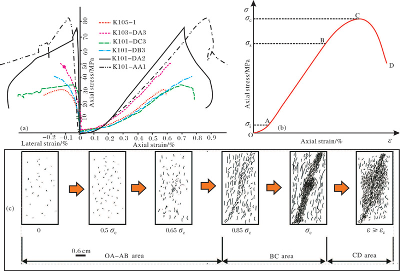 | Fig.6 Uniaxial stress-strain curves of various micro-fractured low-permeability sandstone under cyclic compression loading(a) and evolutionary process from microcracks to macrocracks(b) In area OA-AB few microcracks form, in area BC the rock dilate obviously, producing a large number of microcracks could generate, in area CD series of macrocracks appear, accompanied with the stress declining, fracture density and aperture increasing.Only results up to peak stress and 85 percent of peak stress are included |
(1) Inperiod of compaction by initial damage(OA segment), in Fig.5b, c, the microcracks in porous rocks began to close with compression, allowing rocks to become dense, fracture aperture to reduce significantly and permeability to die away gradually.
(2) AB segmenton stress-strain curve presents proximate straight line feature, during which rock occurs elastic deformation with few obvious extensional fractures appearing, although axial strain increases significantly, unlike studies on carbonate samples of middle Tarim area by Song[34]and Gale[55]. Under this condition, mutually parallel or nearly parallel extensional fractures are not developed here, as most of microcracks belong to intragranular fracture type on surface of the particles, with aperture less than 0.001 mm and extended distance less than 0.2 mm. Overall, in this stage, there develop few fractures, which present scattered in distribution and seem grid and directionless trading.
(3) The BC segment in Fig.5b is no longer a straight line, with increasing strain on radial, which is considered as a dilatation stage. As the yield limit of the rock, the stress of point B is equal to 0.85 σ c, after this point, fracture number increases rapidly and are of strong orientation and approximately equal in distances, all of which prove that fractures tend to develop along anisotropy when the angle between pre-existing microcracks and σ 1 is low(< 30° ).
(4) While stress reaches the peak strength (point C) (Fig.5b), the overall macro-rupture occurs, along with the serious decrease of stress and significant increase of strain.
(5) Breakdown of sandstoneas evolution result of intragranular microcracks, mainly includes development of original microcracks, aggregation of microcracks, interconnection of macrocracks. From above, it can be indicated that a large number of new fractures appeared at the compressive stress equaling to 0.85 σ c, which can be defined as an indication or precursor for microcracks to sprout and develop during loading. Xia et al.[56]conducted uniaxial compression experiment on MTS with sandstone samples under various stress conditions, and found that microcracks increased as stress boosted, especially when stress reached or exceeded 0.85 σ c, the number of fractures exploded instantaneously and the number of large-scale fractures (length > 0.4 mm) increased faster than that of small-scale fractures (length≤ 0.3 mm), meanwhile the number of fractures with small angle of≤ 30° with respect to principal stress increased faster than that of fractures with large angle of> 30° (Fig.4).
According torock mechanics theory[57], geo-stresses, important influencing factors of the stability of the deep rock mass, are the main factors controlling development of fractures in crust, which is characterized by three-dimensional state of stress including two horizontal principal stresses(σ H and σ h) and a vertical principal stress(σ v) in most conditions. In the stress field, if the rock appears distorted as time passes and much elastic strain energy accumulates everywhere; the energy intensity usually can be characterized by rock’ s strain energy per unit volume, which is strain energy density[58].
Where
Combing Eq.(7), Eq.(8), Eq.(9) with Eq.(6), new strain energy density is given by
Where ε is the strain, μ is the Poisson’ s ratio.
Theoritically, low-permeability sandstone is characterized by strong brittleness, according to brittle fracture mechanics theory and maximum tensile stress theory, when elastic strain energy release rate accumulating in brittle rocks which is equals to the energy per unit volume for generating fractures, rocks will break. Especially the fine sandstone and mid-fine sandstone in Kela-2 area, when surrounding three-dimensional stress state reaches the rock strength, macro brittle fractures will occur with strain energy releasing, part of which will offset the surface energy of new fractures, the rest of which will offset in form of elastic waves[59]. However, for fractures, the elastic wave energy is so weak that can be completely ignored, so we assume that all of fractures in rocks are caused by the releasing energy, here law of conservation of energy must be abided.
Where Dvf is fracture volume density per unit volume (m2/m3);
In Eq.(11) if
Where
In most cases, there exist three types of stress environment in earth crust, such as type Ia, type II and type III, and, different mechanical behaviors appear under different stress state, for example, shear fractures probably form in the extrusion conditions and extensional fractures probably form in the extension environment, so individual condition must be discussed respectively.
As stated above, 0.85 σ c as peak period for the initiation of fracture swarm, its corresponding strain density energy is close to
| Table 3 Strain energy parameters of four specimens in Kela-2 area |
Taking average of J in Table 3 to acquire
In order to test and verify the reliability of
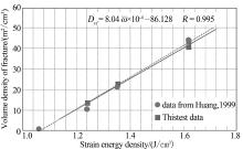
Where the correlation coefficient reaches 0.995, and the relative errors for coefficients a and b by two different methods are 12.6% and 17.3% respectively, both within allowed error range. And it should bepointed out that regardless of the rock is intact or fractured, the fitting curve exhibits positive linear relationship between parameters. Even if there is a small devi-ation, the main reasons still can be caused by aniso- tropic mechanical properties, i.e. combination of pre-existing weakness planes and unruptured rocks. Whatever it takes, conforming
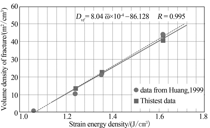 | Fig.7 Linearized relational graphs between strain energy density and fracture volume density at key stress point (0.85 σ c) based on stress strain curves The data from reference[60] and the experimental results showed good agreement |
As has been proved by the experiments, relationship between strain energy density and fracture volume density under complex state of stress is unlike that under unaxial state of stress, without popularity in practice. In the former case, elastic strain energy
| Table 4 Stress-strain state and fracture parameters of rocks in experiments |
If the minimum principal stress σ 3 is given, and σ 3≥ 0 MPa under triaxial state of stress (in contrast σ 3< 0 MPa representing tensile state of stress), using above-mentioned failure criteria, we get the minimum value of maximum principal stress for rock failure.
In fact, the calculatedσ 1 does not represent actual maximum principal stress, but exactly equals bursting stress σ 3, here for the later convenience, we try using σ p to replace σ 1.
Under any stress state σ ij=
Combining Eq.(12) and Eq.(13) we get
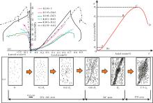
Combining previous research results, in study area, there is no clear relationship between poisson’ s ratio and confining pressure, however, clear linear relationship is discovered between strength, elastic modulus and confining pressure through a lot of experimental data, and further analysis demonstrate that there appears a linear relationship between compressive strength and elastic modulus despite of the great change of confining pressure and difference in unaxial compression strength(Fig.8a), which can be expressed as
Where φ is the internal friction angle, C0 is the cohesive strength of rocks.
Putting Eq.(19) and Eq.(17) into Eq.(18), Eq.(18) is simplified to
Undoubtedly, under confining pressure conditions, energy accumulated in the rocks not only must overcome the molecular internal cohesive forces, but also spares part of its own to resist confining pressure, as a result, the needed power for fractures per unit area increase in progress, a comprehensive superposition result is given by
Where J0 is fracture surface energy without confining pressure or under unaxial compressive stress (J/m2), Δ J is the additional surface energy caused by confining pressure σ 3 (J/m2), μ is Poisson’ s ratio.
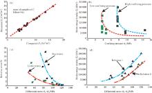
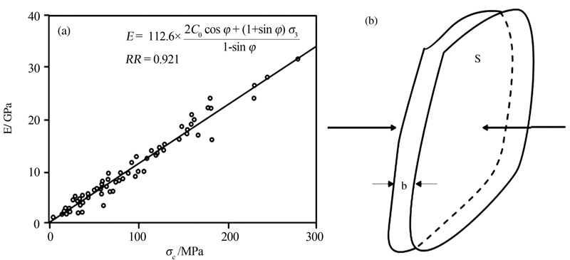 | Fig.8 Main controlling factors for variation of fracture parameters under various confining pressure (a) Linearized relationship between compressive strength and elastic modulus under confining pressure in Kela-2 area. (b)Relation diagram between fracture surface energy and confining pressure at depth. Unlike the unaxial compression condition, there will consume a certain amount of extra energy to resist confining pressure, the higher the confining pressure, the higher the fracture surface energy |
Now we assume a default fracture with aperture b, area S and confining pressure σ 3(Fig.8b), then work of σ 3 for the fracture is defined by
Where Δ J=
Combing Eq.(20), Eq.(21)and Eq.(23) into Eq.(12), we can get the fracture volume density.
Dvf=
To determine the value of σ p, some conversions are needed based on Eq.(24), with experiments, there σ p=σ 1 and strain is given, the above equations are equivalent to
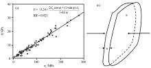
To verify the validity of aboveequations or mechanical models, firstly we use Eq.(25) to compute fracture volume density, then a comparison is carried out by actual data in the study area. It is necessary to emphasize that some of original data is drawn from the triaxial test results of sandstone in Fig.9.
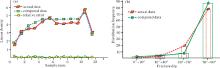
Totally therelative errors of 94.11% of samples are less than 15%, demonstrating the accuracy and practicability of the models (Fig.8). Meanwhile through detailed statistics between computed results and measured data, several major laws have been found out. Firstly, with the increase of σ 3 or confining pressure,
In order to meet the demands of the real reservoir development behind, linear fracture density in low-permeability sandstone is needed as well as fracture surface density with respect to the calculated model of fracture volume density Dvf. If stress σ 1 is tilted horizontally by an angle θ from the fracture plane, the linear fracture density is calculated as follows
Dlf=
Where Dlf is linear fracture density (1/m), L1, L2, L3 are respectively the lengths in directions of σ 1, σ 2 and σ 3(m) in Representative Elementary Volume(REV).
If stress σ 1 is parallel to fracture plane, the linear fracture density is calculated as follows
Dlf=Dvf (27)
In extensional basins, there always exists type Ib of stress state which is usually with one horizontal principal stress negative(tensile) and the other positive(compressive), both are small within several MPa. In contrast, when the rocks remain in the vertical stress which is positive, till to ground surface the compressional force gets small enough to be neglected[61]. From perspective of rock mechanics, as nearing the ground surface, the stress has become smaller, under the state dominated by one or two extensional principal stress, there must appears σ 3< 0, at this time the appropriate applied fracture criteria is not Mohr-Coulomb criterion but Griffith criterion, and the foundation of corresponding stress-strain relationship also has a bit difference from the above.
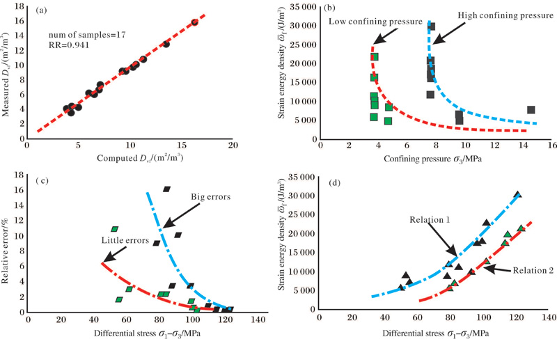 | Fig.9 Comparison between computed results and actual measured data of fracture density (a)The relative errors between measured volume density of fracture by drill cores and calculated density by mechanical model range from 0.22 percent to 10.87 percent, local error up to 20%, which shows good reliability.(b)A clear boundary in confining pressure Ca. 8 MPa exists to divided relation curves into two areas, i.e. low confining pressure area and high confining area.(c)The higher the differential stress(σ 1-σ 3), the larger the relative errors. (d) The higher the differential stress(σ 1-σ 3), the bigger the strain energy density, and both relation curves the two curves parallel to each other with same slope |
Certainly, under extension state, rock appears stronger brittle deformation than that of compression state, such as stress and strain which are good linear relationship before peak strength, after that, rock strength rapidly decreases to zero without any precursor microcracks. By contrast, under compression state around peak strength value, rock normally undergoes several deformation stages with noticeable precursor microcracks and residual strength, and the total accumulated strain from beginning is also bigger than that of the former.
In conclusion, when tension stress appears, rock preferred occurring tension fracture or tension-shear composite fracture approximately perpendicular to the maximum principal stress, at this time, an essential thing must be satisfied that the elastic strain energy density
Throughout theexperiments, σ t, E and the ultimate strain ε t are acquired now, then
Finally we can get the fracture volume density:
According tothe above description, when(σ 1+3σ 3)> 0, by Griffith criterion, there should have
cos2θ =
θ =
When(σ 1+3σ 3)≤ 0, θ =0, we get
Dlf=Dvf (31)
As we all know, in three-dimensional in-situ stress system of coordinates, thecalculation of fracture strike and dip depends on reasonable projection, e.g. axes-x agrees with east-west direction, axes-y agrees with north-south direction, axes-z agrees with vertical direction. Thus, the strike angle α in the x-y plane can be characterized by its normal vector of fracture surface. Here
if 0≤ α Y< 90° , α =90° -α Y (32)
if 90° < α Y< 0, α =(-90° -α Y)+360° (33)
In three-dimensional in-situ stress system of coordinates, inclination angle α dip between the lx+my+nz=0 plane and y=0 plane is assumed as the inclination angle between fracture surface and x-y plane, which is given by
cosα dip=
=
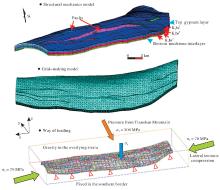
The modeling approach was used in this study by utilizing the Finite Element (FE) technique, and geomechanical models will be run in order to simulate the stress distribution for further predicting fracture development and distribution. The general-purpose finite element code Ansys was selected for this study because it is well-suited to analyzing geomechanical problems over a wide range of scales in one, two and three dimensions. The initial three-dimensional model geometries were constructed based on the restored geologic section constrained by field measurements, and incorporated the generalized mechanical stratigraphy (the gypsum, sandstone and mudstone member, E1k; fine sandstone, medium sandstone, muddy siltstone, K1bs1; medium sandstone, siltstone, fine sandstone, mudtone, K1bs2; medium sandstone, fine sandstone, pebbly sandstone, muddy siltstone, K1bs3)(Fig.11a). All model layers were discretized using primarily three-node triangle plane strain elements with some four-node quadrilateral elements (approximately 311226 total elements in the model).
Besides, based upon the field observations in the Kuqa Depression and some studies of smart[4] and Ju et al.[22], meanwhile combining a series of compressional conjugated fractures, the maximum tectonic stress direction in the area at the stage of Himalayan Orogeny was nearly S-N, and was about 300 MPa. Then based on paleotectonic deformation, a methodology including inverse and forward method is used to investigate minimum paleostress field, which was about 70 MPa.Thus in the first step we elected to set southern edge(hinterland side) in the simulated stratigraphy for fixed boundary so that Kela-2 anticline could uplift if the stress state was appropriate. The deformation was imposed in a second step with thrusting simulated by a displacement boundary condition along the foreland (north) side of the model to simulate the deformation of a fault-related fold. The base of the model was pinned, and a gravity load was applied to the entire model domain and the system was allowed to reach equilibrium.
Base on the above mechanics experiments, the material properties are assigned to the elements representing the various lithologies. The mechanical properties of rocks influence the deformation and stress distribution, thus an mechanics experiment of rock is needed to support the mechanical parameters (the density, Young’ s modulus, Poisson’ s ratio, friction angle and cohesion) for the present Kela-2 fault-related fold geo mechanical model[28]. However, the site-specific material properties are not available for all the stratigraphic layers being modeled completely(Table 5), values of boundary master faults are selected from the literatures[10], for simplicity, the density, Young’ s modulus, Poisson’ s ratio is set to 2.35 g/cm3, for each layer respectively.
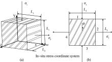
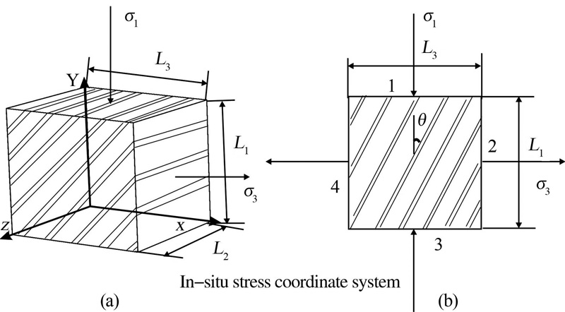 | Fig.10 In-situ stress coordinate system representing fracture distribution and differential stress (σ 1-σ 3) plane based on an Element volume (a)An Element Volume(REV)is selected to establish the relationship between stress and fracture parameters under complex stress condition, and some hypothesis is made as follows: ①It is so small enough to be easily cut through; ②The scattered microcracks inner element can be negligible; ③The element is supposed as a parallel epipedon with sides L1, L2, L3, here we specify the compression stress positive and σ 1> σ 2> σ 3, thus the σ 1 corresponding with side L1, the corresponding σ 2 with side L2, the t corresponding σ 3 with the side L3.(b)Transection perpendicular to σ 2, namely (σ 1-σ 3) plane |
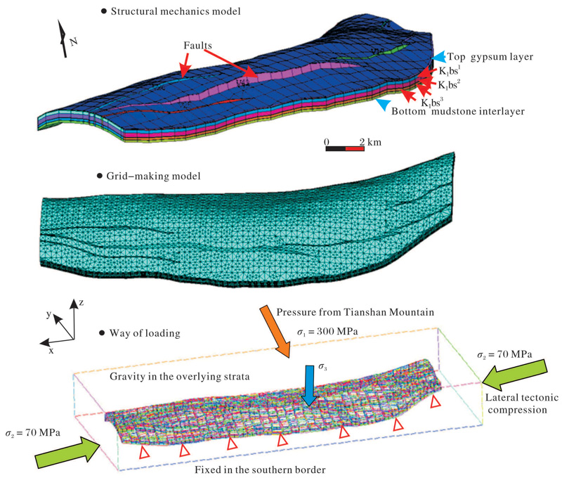 | Fig.11 Initial geometry, boundary conditions and meshing grid of the finite element model. Red triangle indicate fixed boundary, filling arrows indicate direction of force |
| Table 5 Material properties used in the Kela-2 reservoir geomechanical model |
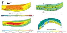
Results from finite element method including predicting paleostress and spatial distribution of linear fracture density show that fractures often develop around anticlinal core, and development intensity of conjugated fractures is positively correlated with regional stress intensity, however, fracture density is relatively lower araund fault zones(Fig.12), which just shows the cracking of low-permeability sandstones are mainly caused by local stress and strain perturbations in the uplifting process of anticline instead of perturbations by the secondary faults. The distribution map of fracture strike reveals that most of shear conjugated fractures with strike ranging from NNW-NNE sporadically distribute in north and south wing of kela-2 anticline and the nearly EW striking fractures intensively distribute along the long axis of the anticline. Moreover, prediction results show that the natural fracture networks tend to be heterogeneous and messy near formation or lithology interfaces, where the sandstone mutates into mudstone, and fractures are clustered in swarms and irregularly distributed(Fig.12d).
As shown in the wells (Fig.13), the overall geomechanical finite element modeling results are in agreement with core observation result and FMI result. The fracture density of Well 202 and Well 204 measuring point in K1bs2 is as high as 0.124~1.274 m-1 and 3.277 m-1 in the core and FMI, and the values of calculated density corresponding to these two points in the model are 1.8~2.8 m-1 and 2.4~3.4 m-1 respectively. Comparison results based on 12 sample spots in Bashijiqiuke Formation show that there is little error between computed result and actual data from cores and microscopic observations, especially in terms of fracture linear density, most relative errors of samples are within 0.15, and the relatively larger ones distribute randomly. From evaluation of cores, the predominating fracture type is high angle cracks with dip mostly greater than 70° , and high angle fracture type is less developed, low angle fracture type occupies the least proportion, all of which is very consistent with the calculations(Fig.13).
 | Fig.12 Simulation results of paleo stress field and linear fracture distribution calculated from geomechanical model in K1bs2 Negative values in the stress diagram represent compression stress, and positive values represent tension stress |
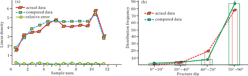 | Fig.13 Comparison of fracture parameters between computed results and actual data in Kela-2 reservoir |
An adaptedgeomechanical method is used to calculate the fracture parameters governing the development of the low-permeability sandstone reservoirs for unconventional resources. This method is more applicable than other methods for developed fracture area after multiphase tectonic movements and more readily modified to fit the finite element modelling and calculation, which also agrees well with the present core observations.
From the rock mechanics experiments under cyclic loading, crack evolution of low-permeability sandstone(maybe contain a small amount of microcracks) is summed up to three stages, i.e. initial compaction stage, propagation stage and coalescence stage extracted from three-dimensional μ CT scan. When reach peak strength, namely 0.85 σ c, rocks will occur volume expansion and microcracks will rapidly connect each other, this key value is recorded, exactly equaling to another key value τ =0.85 σ c(σ c< 200 MPa), which is the critical sliding value mentioned in Byerlee law. From microcosmic point of view, there only exists three failure models in brittle rocks: Shear fracturing, tensional fracturing, and composite fracturing, which mainly depend on confining pressure, principal stress intensity and pre-existing weakness plane, etc. In addition, spacing of fractures is also an important factor to influence strength of fractureed rocks, but if multiple sets of cracks exist, the strength can be replaced by equivalent strength or measured through mechanical tests directly. After a lot of experiments and testing researches, a relationship between fracture volume density and stress-strain of low-permeability sandstone reservoirs is finally established, as a result, expressions or geomechanical models have been obtained to characterize fracture parameters after various tectonic movements under different stress states. And this method can be changed into a program running on finite element simulation platform, which has become a popular and effective modeling approach in the prediction of the generation of fractures and their spatial distribution. However, the geomechanical model is limited to the strength prediction for fractured anisotropic rocks and triaxial testing conditions. Further study is needed to extend the composite modi-ed criterion for anisotropic rock masses and polyaxial testing conditions with emphasis on the effect of diffused heterogenous pre-existing fractures. It will be worth while somehow if the geomechanical model for fracture volume density could be comprehensive to consider the energy of plastic deformation and to predict strength of transversely isotropic rocks in different directions of weakness planes with limited data in one direction.
The authors have declared that no competing interests exist.
| [1] |
|
| [2] |
|
| [3] |
|
| [4] |
|
| [5] |
|
| [6] |
|
| [7] |
|
| [8] |
|
| [9] |
|
| [10] |
|
| [11] |
|
| [12] |
|
| [13] |
|
| [14] |
|
| [15] |
|
| [16] |
|
| [17] |
|
| [18] |
|
| [19] |
|
| [20] |
|
| [21] |
|
| [22] |
|
| [23] |
|
| [24] |
|
| [25] |
|
| [26] |
|
| [27] |
|
| [28] |
|
| [29] |
|
| [30] |
|
| [31] |
|
| [32] |
|
| [33] |
|
| [34] |
|
| [35] |
|
| [36] |
|
| [37] |
|
| [38] |
|
| [39] |
|
| [40] |
|
| [41] |
|
| [42] |
|
| [43] |
|
| [44] |
|
| [45] |
|
| [46] |
|
| [47] |
|
| [48] |
|
| [49] |
|
| [50] |
|
| [51] |
|
| [52] |
|
| [53] |
|
| [54] |
|
| [55] |
|
| [56] |
|
| [57] |
|
| [58] |
|
| [59] |
|
| [60] |
|
| [61] |
|